
Inverse_propensity_weighting_&_doubly_robust_estimation
Propensity Scores in Practice
A fully commented, marketing-focused notebook
Goal of this notebook
This notebook is designed to teach Chapter 5 of Matheus Facure – Causal Inference in Python, not just run code.
You will see:
- Why naive analysis is biased
- How propensity scores fix selection bias
- When IPW breaks
- Why Doubly Robust (DR) is safer
- How Double Machine Learning fits conceptually
- How to explain results to business / MRM stakeholders
We use a public marketing dataset (Hillstrom email campaign) so the ideas map directly to real-world marketing analytics
📊 Hillstrom (MineThatData) Email Marketing Dataset
Direct download (CSV): https://raw.githubusercontent.com/W-Tran/uplift-modelling/master/data/hillstrom/Kevin_Hillstrom_MineThatData_E-MailAnalytics_DataMiningChallenge_2008.03.20.csv
You can:
Open this link directly in a browser
Or use it in Python with pd.read_csv(url)
🔗 Original source (background & documentation)
MineThatData – Email Analytics Challenge (Kevin Hillstrom): https://www.minethatdata.com/data-mining-challenge/
Big Picture (context)
We want to answer a causal question:
Does sending a marketing email cause higher customer spend / conversion?
This is not the same as:
“Do customers who receive emails spend more?”
Why?
- Marketing emails are not sent at random
- Better / more engaged customers are more likely to be targeted
- That creates selection bias
Chapter 5 is about how to remove that bias.
Methods we will compare
We will implement and compare four approaches:
- Naive regression – shows the bias
- IPW (Inverse Propensity Weighting) – design-based correction
- Outcome regression – model-based correction
- Doubly Robust (AIPW) – combines both
- Conceptual Double ML – how DR extends to ML safely
For each method, we answer:
- What assumption does it rely on?
- When does it work?
- When does it fail?
Dataset: Hillstrom Email Marketing (Public)
This dataset comes from a well-known marketing challenge.
Interpretation of columns
- Each row = one customer
segment= which email (if any) the customer received- Customer attributes = recency, history, channel, etc.
- Outcomes = spend and conversion
Treatment definition
T = 1→ customer received any emailT = 0→ customer received no email
This mirrors real-world campaign targeting.
# === Standard imports ===
# We keep models simple and interpretable on purpose.
# Chapter 5 is about *causality*, not model tuning.

import numpy as np
import pandas as pd
import matplotlib.pyplot as plt

from sklearn.model_selection import train_test_split
from sklearn.compose import ColumnTransformer
from sklearn.preprocessing import OneHotEncoder
from sklearn.pipeline import Pipeline
from sklearn.linear_model import LogisticRegression, LinearRegression
from sklearn.metrics import roc_auc_score

np.random.seed(42)
# === Load the Hillstrom dataset (public) ===
# If this fails due to network restrictions, download the CSV manually
# and set DATA_PATH accordingly.

import pathlib, urllib.request

DATA_DIR = pathlib.Path("data")
DATA_DIR.mkdir(exist_ok=True)
DATA_PATH = DATA_DIR / "hillstrom.csv"

URL = "https://raw.githubusercontent.com/W-Tran/uplift-modelling/master/data/hillstrom/Kevin_Hillstrom_MineThatData_E-MailAnalytics_DataMiningChallenge_2008.03.20.csv"

if not DATA_PATH.exists():
    urllib.request.urlretrieve(URL, DATA_PATH)

df = pd.read_csv(DATA_PATH)
df.head()
| recency | history_segment | history | mens | womens | zip_code | newbie | channel | segment | visit | conversion | spend | |
|---|---|---|---|---|---|---|---|---|---|---|---|---|
| 0 | 10 | 2) $100 - $200 | 142.44 | 1 | 0 | Surburban | 0 | Phone | Womens E-Mail | 0 | 0 | 0.0 |
| 1 | 6 | 3) $200 - $350 | 329.08 | 1 | 1 | Rural | 1 | Web | No E-Mail | 0 | 0 | 0.0 |
| 2 | 7 | 2) $100 - $200 | 180.65 | 0 | 1 | Surburban | 1 | Web | Womens E-Mail | 0 | 0 | 0.0 |
| 3 | 9 | 5) $500 - $750 | 675.83 | 1 | 0 | Rural | 1 | Web | Mens E-Mail | 0 | 0 | 0.0 |
| 4 | 2 | 1) $0 - $100 | 45.34 | 1 | 0 | Urban | 0 | Web | Womens E-Mail | 0 | 0 | 0.0 |
# === Define treatment, outcome, and covariates ===

df = df.copy()

# Treatment: received any email vs none
df["T"] = (df["segment"].str.lower() != "no e-mail").astype(int)

# Outcomes
df["Y_spend"] = df["spend"].astype(float)
df["Y_conv"] = df["conversion"].astype(int)

# Covariates (chosen to reflect realistic marketing features)
covariates = [
    "recency", "history", "history_segment",
    "mens", "womens", "zip_code", "newbie", "channel"
]

df[covariates + ["T", "Y_spend", "Y_conv"]].head()
| recency | history | history_segment | mens | womens | zip_code | newbie | channel | T | Y_spend | Y_conv | |
|---|---|---|---|---|---|---|---|---|---|---|---|
| 0 | 10 | 142.44 | 2) $100 - $200 | 1 | 0 | Surburban | 0 | Phone | 1 | 0.0 | 0 |
| 1 | 6 | 329.08 | 3) $200 - $350 | 1 | 1 | Rural | 1 | Web | 0 | 0.0 | 0 |
| 2 | 7 | 180.65 | 2) $100 - $200 | 0 | 1 | Surburban | 1 | Web | 1 | 0.0 | 0 |
| 3 | 9 | 675.83 | 5) $500 - $750 | 1 | 0 | Rural | 1 | Web | 1 | 0.0 | 0 |
| 4 | 2 | 45.34 | 1) $0 - $100 | 1 | 0 | Urban | 0 | Web | 1 | 0.0 | 0 |
Step 1 — Why naive analysis fails
We start with the wrong approach on purpose.
If we simply compare:
- average spend of emailed customers
- vs non-emailed customers
we are implicitly assuming random assignment.
That assumption is false in observational marketing data.
👉 This step is crucial for storytelling:
it shows stakeholders why causal methods are needed.
# === Naive comparison (intentionally biased) ===

naive_spend = df.groupby("T")["Y_spend"].mean()
naive_conv  = df.groupby("T")["Y_conv"].mean()

print("Naive spend difference:", naive_spend[1] - naive_spend[0])
print("Naive conversion difference:", naive_conv[1] - naive_conv[0])

# Interpretation:
# This looks like a treatment effect,
# but it mixes true causal impact with selection bias.
Naive spend difference: 0.5967960667278982
Naive conversion difference: 0.004954571155268468
Step 2 — Propensity Scores (the key idea of Chapter 5)
The propensity score is:
[ e(X) = P(T=1 | X) ]
Plain English:
“Given what we know about a customer, how likely were they to be emailed?”
Why this matters:
- Customers with the same propensity score are comparable
- Conditioning on the propensity score balances all covariates
This is the foundation of IPW and DR.
# === Propensity score model ===

X = df[covariates]
T = df["T"].values

num_cols = [c for c in covariates if pd.api.types.is_numeric_dtype(df[c])]
cat_cols = [c for c in covariates if c not in num_cols]

preprocess = ColumnTransformer(
    [
        ("num", "passthrough", num_cols),
        ("cat", OneHotEncoder(handle_unknown="ignore"), cat_cols),
    ]
)

ps_model = Pipeline(
    [
        ("prep", preprocess),
        ("logit", LogisticRegression(max_iter=2000)),
    ]
)

X_train, X_test, T_train, T_test = train_test_split(
    X, T, test_size=0.3, stratify=T, random_state=42
)

ps_model.fit(X_train, T_train)
e_hat = ps_model.predict_proba(X_test)[:, 1]

print("Propensity AUC:", roc_auc_score(T_test, e_hat))
Propensity AUC: 0.49176685713090773
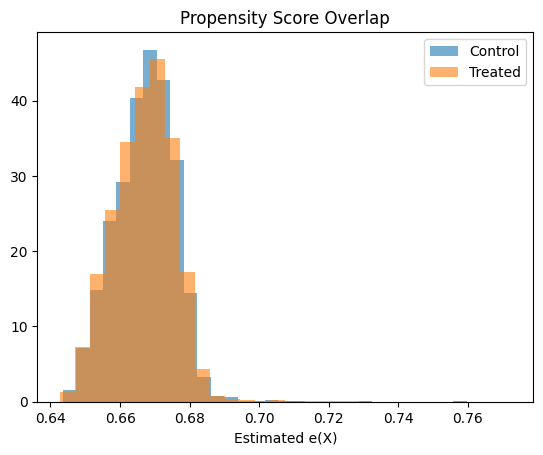
# === Overlap / positivity check ===

plt.hist(e_hat[T_test == 0], bins=30, alpha=0.6, label="Control", density=True)
plt.hist(e_hat[T_test == 1], bins=30, alpha=0.6, label="Treated", density=True)
plt.legend()
plt.title("Propensity Score Overlap")
plt.xlabel("Estimated e(X)")
plt.show()

# Interpretation:
# Good overlap → IPW is feasible
# Poor overlap → expect unstable weights
Step 3 — IPW (Inverse Propensity Weighting)
Core idea
Instead of changing the model, we change the importance of observations.
- Customers who were unlikely to be emailed but were emailed → get large weight
- Customers who were very likely to be emailed → get small weight
This creates a pseudo-randomized dataset.
Key assumption
- The propensity model is correct
# === IPW estimator ===

def ipw_ate(y, t, e, stabilized=False):
    eps = 1e-6
    e = np.clip(e, eps, 1 - eps)

    if stabilized:
        p = t.mean()
        w = np.where(t == 1, p / e, (1 - p) / (1 - e))
    else:
        w = np.where(t == 1, 1 / e, 1 / (1 - e))

    ate = (
        np.sum(w[t == 1] * y[t == 1]) / np.sum(w[t == 1])
        - np.sum(w[t == 0] * y[t == 0]) / np.sum(w[t == 0])
    )
    return ate, w

Y = df.loc[X_test.index, "Y_spend"].values

ate_ipw, w_raw = ipw_ate(Y, T_test, e_hat, stabilized=False)
ate_ipw_stab, w_stab = ipw_ate(Y, T_test, e_hat, stabilized=True)

print("IPW ATE:", ate_ipw)
print("Stabilized IPW ATE:", ate_ipw_stab)
IPW ATE: 0.6869934772562071
Stabilized IPW ATE: 0.6869934772562072
Step 4 — Why IPW can be dangerous
IPW can fail badly when:
- Some customers have propensity scores near 0 or 1
- Weights explode
- A few customers dominate the estimate
We will:
- Inspect weight distributions
- Compute effective sample size (ESS)
- Apply stabilization and clipping
This is mandatory in real work.
# === Weight diagnostics ===

def ess(w):
    return (w.sum() ** 2) / (w ** 2).sum()

print("Max raw weight:", w_raw.max())
print("ESS raw:", ess(w_raw))
print("ESS stabilized:", ess(w_stab))

# Interpretation:
# Stabilization usually increases ESS dramatically
Max raw weight: 4.160191208753913
ESS raw: 17043.204198395597
ESS stabilized: 19193.43392200713
Step 5 — Doubly Robust Estimation (AIPW)
This is the main takeaway of Chapter 5.
Doubly Robust combines:
- A propensity model (design-based)
- An outcome model (model-based)
Why it’s powerful
- If either model is correct → estimate is consistent
- You get two chances to be right
This is why DR is the default choice in practice.
# === Outcome regression ===

outcome_model = Pipeline(
    [
        ("prep", preprocess),
        ("lr", LinearRegression()),
    ]
)

outcome_model.fit(
    pd.concat([X_train, pd.Series(T_train,index=X_train.index, name="T")], axis=1),
    df.loc[X_train.index, "Y_spend"],
)

# Simpler demonstration:
# Separate models by treatment group

m1 = LinearRegression().fit(
    preprocess.fit_transform(X_train[T_train == 1]),
    df.loc[X_train.index[T_train == 1], "Y_spend"]
)

m0 = LinearRegression().fit(
    preprocess.fit_transform(X_train[T_train == 0]),
    df.loc[X_train.index[T_train == 0], "Y_spend"]
)

m1_hat = m1.predict(preprocess.transform(X_test))
m0_hat = m0.predict(preprocess.transform(X_test))

ate_or = (m1_hat - m0_hat).mean()
print("Outcome regression ATE:", ate_or)
Outcome regression ATE: 0.5598623633614704
# === Doubly Robust / AIPW ===

def aipw_ate(y, t, e, m0, m1):
    eps = 1e-6
    e = np.clip(e, eps, 1 - eps)
    return np.mean(
        (m1 - m0)
        + t * (y - m1) / e
        - (1 - t) * (y - m0) / (1 - e)
    )

ate_dr = aipw_ate(Y, T_test, e_hat, m0_hat, m1_hat)
print("Doubly Robust ATE:", ate_dr)

# Interpretation:
# If either the propensity model OR outcome model is correct,
# this estimate is consistent.
Doubly Robust ATE: 0.6886373812888652
Step 6 — Where Double Machine Learning fits
Double ML builds on DR ideas but adds:
- Cross-fitting
- Orthogonalization
- Safe use of ML models
Conceptually:
- DR = robustness to misspecification
- Double ML = robustness + protection against ML overfitting
We explain this conceptually (implementation is similar but heavier).
Final Summary (what to remember)
- Regression trusts the outcome model
- IPW trusts the assignment mechanism
- DR trusts either one
- Double ML lets you use ML safely
In observational marketing data:
Doubly Robust is almost always the right baseline choice.