
Causal_graphs_full_tutorial_networkx
Causal Graphs, Confounding, Colliders, and Selection Bias
A Practical Tutorial Inspired by Chapter 3 (with Original Examples)
This notebook is inspired by Chapter 3 of Matheus Facure’s Causal Inference in Python,
but uses different stories, variables, and numbers so it stands on its own and is safe to share.
We will cover:
- Three basic graphical patterns (chain, fork, collider) and how association flows.
- A more complex product analytics DAG and d-separation using a custom helper on
networkx. - Backdoor paths and confounding with a marketing email & revenue example.
- The adjustment formula with a small toy dataset.
- Selection bias in a feature rating survey, showing how even A/B tests can lie.
We avoid pgmpy completely and implement a small, general-purpose is_d_separated helper using networkx only,
so the notebook is robust to library version issues.
1. Setup and d-separation helper
import numpy as np
import pandas as pd
import matplotlib.pyplot as plt
import networkx as nx

np.random.seed(42)
pd.set_option("display.precision", 4)

def _ancestors(G, nodes):
    """Return all ancestors of a set of nodes in a directed graph G."""
    anc = set()
    stack = list(nodes)
    while stack:
        n = stack.pop()
        for p in G.predecessors(n):
            if p not in anc:
                anc.add(p)
                stack.append(p)
    return anc

def is_d_separated(G, X, Y, Z):
    """
    Check d-separation between sets X and Y given Z in DAG G using
    the moralized ancestral graph method.

    G : networkx.DiGraph
    X, Y, Z : iterables of node labels

    Returns True if X and Y are d-separated given Z, False otherwise.
    """
    X = set(X); Y = set(Y); Z = set(Z)

    # 1. Keep only ancestors of X ∪ Y ∪ Z (plus themselves)
    relevant = set(X) | set(Y) | set(Z)
    relevant |= _ancestors(G, relevant)
    H = G.subgraph(relevant).copy()

    # 2. Moralize: undirected graph, connect parents of each child
    M = nx.Graph()
    M.add_nodes_from(H.nodes())
    # undirected versions of all edges
    for u, v in H.edges():
        M.add_edge(u, v)
    # marry parents
    for child in H.nodes():
        parents = list(H.predecessors(child))
        for i in range(len(parents)):
            for j in range(i + 1, len(parents)):
                M.add_edge(parents[i], parents[j])

    # 3. Remove observed nodes Z
    M.remove_nodes_from(Z)

    # 4. Check if any node in X is connected to any node in Y
    for x in X:
        if x not in M:
            continue
        comp = nx.node_connected_component(M, x)
        if any(y in comp for y in Y):
            return False  # not d-separated (path exists)
    return True  # d-separated

# Quick sanity check on the three basic patterns
if __name__ == "__main__":
    G_chain = nx.DiGraph([("X","M"),("M","Y")])
    print("Chain X,Y | ∅:", is_d_separated(G_chain, {"X"},{"Y"}, set()))       # False
    print("Chain X,Y | M:", is_d_separated(G_chain, {"X"},{"Y"},{"M"}))       # True

    G_fork = nx.DiGraph([("C","X"),("C","Y")])
    print("Fork X,Y | ∅:", is_d_separated(G_fork, {"X"},{"Y"}, set()))        # False
    print("Fork X,Y | C:", is_d_separated(G_fork, {"X"},{"Y"},{"C"}))         # True

    G_col = nx.DiGraph([("X","C"),("Y","C")])
    print("Coll X,Y | ∅:", is_d_separated(G_col, {"X"},{"Y"}, set()))         # True
    print("Coll X,Y | C:", is_d_separated(G_col, {"X"},{"Y"},{"C"}))          # False
Chain X,Y | ∅: False
Chain X,Y | M: True
Fork X,Y | ∅: False
Fork X,Y | C: True
Coll X,Y | ∅: True
Coll X,Y | C: False
2. Three Fundamental Causal Structures
We look at:
- Chain: X → M → Y
- Fork (common cause): X ← C → Y
- Collider (common effect): X → C ← Y
We will use a networkx.DiGraph and our is_d_separated helper to see when variables are
independent or dependent, with and without conditioning.
2.1 Chain: X → M → Y
# Chain: X → M → Y
chain = nx.DiGraph([
    ("X", "M"),
    ("M", "Y"),
])

print("Are X and Y d-separated with NO conditioning?")
print(is_d_separated(chain, {"X"}, {"Y"}, set()))  # Expect False (they are connected through M)

print("\nAre X and Y d-separated GIVEN M? (conditioning on mediator)")
print(is_d_separated(chain, {"X"}, {"Y"}, {"M"}))  # Expect True (conditioning blocks the chain)

print("\nAre X and Y dependent (no conditioning)?", not is_d_separated(chain, {"X"}, {"Y"}, set()))
print("Are X and Y dependent given M?", not is_d_separated(chain, {"X"}, {"Y"}, {"M"}))
Are X and Y d-separated with NO conditioning?
False

Are X and Y d-separated GIVEN M? (conditioning on mediator)
True

Are X and Y dependent (no conditioning)? True
Are X and Y dependent given M? False
Intuition
- No conditioning → X and Y are associated via the path X → M → Y.
- Conditioning on M → you block the path and X and Y become independent in the graph (d-separated).
2.2 Fork: X ← C → Y (Common Cause / Confounder)
# Fork: C is a common cause of X and Y
fork = nx.DiGraph([
    ("C", "X"),
    ("C", "Y"),
])

print("Are X and Y d-separated with NO conditioning?")
print(is_d_separated(fork, {"X"}, {"Y"}, set()))  # Expect False: they share C

print("\nAre X and Y d-separated GIVEN C?")
print(is_d_separated(fork, {"X"}, {"Y"}, {"C"}))  # Expect True: conditioning on C blocks path

print("\nAre X and Y dependent (no conditioning)?", not is_d_separated(fork, {"X"}, {"Y"}, set()))
print("Are X and Y dependent given C?", not is_d_separated(fork, {"X"}, {"Y"}, {"C"}))
Are X and Y d-separated with NO conditioning?
False

Are X and Y d-separated GIVEN C?
True

Are X and Y dependent (no conditioning)? True
Are X and Y dependent given C? False
Here C acts as a confounder:
- Without conditioning, X and Y move together because they both depend on C.
- When you condition on C, you remove that shared variation and X and Y become independent.
- This pattern shows why you need to adjust for confounders in causal inference.
2.3 Collider: X → C ← Y (Common Effect / Selection)
# Collider: C is a common effect of X and Y
collider = nx.DiGraph([
    ("X", "C"),
    ("Y", "C"),
])

print("Are X and Y d-separated with NO conditioning?")
print(is_d_separated(collider, {"X"}, {"Y"}, set()))  # Expect True: collider blocks path

print("\nAre X and Y d-separated GIVEN C?")
print(is_d_separated(collider, {"X"}, {"Y"}, {"C"}))  # Expect False: conditioning opens path

print("\nAre X and Y dependent (no conditioning)?", not is_d_separated(collider, {"X"}, {"Y"}, set()))
print("Are X and Y dependent given C?", not is_d_separated(collider, {"X"}, {"Y"}, {"C"}))
Are X and Y d-separated with NO conditioning?
True

Are X and Y d-separated GIVEN C?
False

Are X and Y dependent (no conditioning)? False
Are X and Y dependent given C? True
Key lesson
- Without conditioning, the path X → C ← Y is blocked at the collider C. X and Y are independent.
- When you condition on C (or on a descendant of C), you create a spurious association between X and Y.
- This is the structural origin of many kinds of selection bias.
3. A Product Analytics DAG: Segments, Ads, UI Experiments, and Churn
Now let’s build a slightly more realistic product analytics DAG.
Nodes:
SEG= user segment (e.g. high-value / low-value)H_ISS= historic issues (number of old tickets)UI_EXP= whether the user is assigned to a new UI experimentAD= ad exposure levelSUPPORT= support team loadFAQ= FAQ visitsCHURN= whether the user churns
product_model = nx.DiGraph([
    ("SEG", "UI_EXP"),
    ("SEG", "AD"),
    ("H_ISS", "UI_EXP"),
    ("AD", "FAQ"),
    ("SUPPORT", "FAQ"),
    ("UI_EXP", "CHURN"),
])
3.1 Collider at UI_EXP: SEG → UI_EXP ← H_ISS
print("Are SEG and H_ISS d-separated with NO conditioning?")
print(is_d_separated(product_model, {"SEG"}, {"H_ISS"}, set()))  # Expect True

print("\nAre SEG and H_ISS d-separated GIVEN UI_EXP?")
print(is_d_separated(product_model, {"SEG"}, {"H_ISS"}, {"UI_EXP"}))  # Expect False

print("\nAre SEG and H_ISS dependent (no conditioning)?",
      not is_d_separated(product_model, {"SEG"}, {"H_ISS"}, set()))
print("Are SEG and H_ISS dependent given UI_EXP?",
      not is_d_separated(product_model, {"SEG"}, {"H_ISS"}, {"UI_EXP"}))
Are SEG and H_ISS d-separated with NO conditioning?
True

Are SEG and H_ISS d-separated GIVEN UI_EXP?
False

Are SEG and H_ISS dependent (no conditioning)? False
Are SEG and H_ISS dependent given UI_EXP? True
Here UI_EXP is a collider between SEG and H_ISS.
If you analyze only users in the experiment (conditioning on UI_EXP=1), you can create fake dependence between segment and historic issues.
3.2 Collider at FAQ: AD → FAQ ← SUPPORT
print("Are AD and SUPPORT d-separated with NO conditioning?")
print(is_d_separated(product_model, {"AD"}, {"SUPPORT"}, set()))  # Expect True

print("\nAre AD and SUPPORT d-separated GIVEN FAQ?")
print(is_d_separated(product_model, {"AD"}, {"SUPPORT"}, {"FAQ"}))  # Expect False

print("\nAre AD and SUPPORT dependent (no conditioning)?",
      not is_d_separated(product_model, {"AD"}, {"SUPPORT"}, set()))
print("Are AD and SUPPORT dependent given FAQ?",
      not is_d_separated(product_model, {"AD"}, {"SUPPORT"}, {"FAQ"}))
Are AD and SUPPORT d-separated with NO conditioning?
True

Are AD and SUPPORT d-separated GIVEN FAQ?
False

Are AD and SUPPORT dependent (no conditioning)? False
Are AD and SUPPORT dependent given FAQ? True
Again, FAQ is a collider: users who hit FAQ a lot are more likely to have either high ad exposure or high support load (or both).
Conditioning on FAQ visit can create spurious relationships between AD and SUPPORT.
3.3 Chain H_ISS → UI_EXP → CHURN
print("Are H_ISS and CHURN d-separated with NO conditioning?")
print(is_d_separated(product_model, {"H_ISS"}, {"CHURN"}, set()))  # Expect False

print("\nAre H_ISS and CHURN d-separated GIVEN UI_EXP?")
print(is_d_separated(product_model, {"H_ISS"}, {"CHURN"}, {"UI_EXP"}))  # Expect True

print("\nAre H_ISS and CHURN dependent (no conditioning)?",
      not is_d_separated(product_model, {"H_ISS"}, {"CHURN"}, set()))
print("Are H_ISS and CHURN dependent given UI_EXP?",
      not is_d_separated(product_model, {"H_ISS"}, {"CHURN"}, {"UI_EXP"}))
Are H_ISS and CHURN d-separated with NO conditioning?
False

Are H_ISS and CHURN d-separated GIVEN UI_EXP?
True

Are H_ISS and CHURN dependent (no conditioning)? True
Are H_ISS and CHURN dependent given UI_EXP? False
Here UI_EXP is a mediator on the path from H_ISS to CHURN.
Conditioning on UI_EXP blocks the chain and removes the association.
4. Backdoor Paths and Confounding: Email Campaign & Revenue
Now we show confounding with a compact marketing example.
Variables:
revenue_prev– previous month’s revenueemail_campaign– binary flag: 1 if the customer was targetedrevenue_next– next month’s revenue
Causal story:
- Higher
revenue_prevcustomers are more likely to be targeted. - Higher
revenue_prevalso predicts higherrevenue_next. - The email may give a modest lift to
revenue_next.
marketing_model = nx.DiGraph([
    ("revenue_prev", "email_campaign"),
    ("revenue_prev", "revenue_next"),
    ("email_campaign", "revenue_next"),
])

# To see if there is a noncausal backdoor path from email_campaign to revenue_next,
# we conceptually remove the direct arrow email_campaign → revenue_next
marketing_severed = nx.DiGraph([
    ("revenue_prev", "email_campaign"),
    ("revenue_prev", "revenue_next"),
])

print("Are email_campaign and revenue_next d-separated in the severed graph?")
print(is_d_separated(marketing_severed, {"email_campaign"}, {"revenue_next"}, set()))

print("\nAre they still dependent (backdoor path exists)?",
      not is_d_separated(marketing_severed, {"email_campaign"}, {"revenue_next"}, set()))
Are email_campaign and revenue_next d-separated in the severed graph?
False

Are they still dependent (backdoor path exists)? True
Because of the common cause revenue_prev, even after we conceptually remove the direct causal arrow,
email_campaign and revenue_next are still connected through a backdoor path.
That means there is confounding, and naive comparisons will be biased.
5. Adjustment Formula with a Toy Dataset
Let’s build a tiny dataset of six customers to show how the adjustment formula works in practice.
df = pd.DataFrame({
    "revenue_prev":   [200, 200, 200, 800, 800, 800],
    "email_campaign": [0,   0,   1,   0,   1,   1],
    "revenue_next":   [210, 220, 245, 820, 860, 870],
})
df
| revenue_prev | email_campaign | revenue_next | |
|---|---|---|---|
| 0 | 200 | 0 | 210 |
| 1 | 200 | 0 | 220 |
| 2 | 200 | 1 | 245 |
| 3 | 800 | 0 | 820 |
| 4 | 800 | 1 | 860 |
| 5 | 800 | 1 | 870 |
5.1 Naive Difference (ignoring revenue_prev)
naive_effect = (df.loc[df.email_campaign == 1, "revenue_next"].mean() -
                 df.loc[df.email_campaign == 0, "revenue_next"].mean())
print("Naive difference (campaign - no campaign):", naive_effect)
Naive difference (campaign - no campaign): 241.66666666666669
This naive comparison mixes:
- The true causal effect of the campaign, and
- The fact that higher-revenue customers are more likely to be targeted.
So it is biased upward.
5.2 Stratified Effect (adjusting for revenue_prev)
avg = (df
        .groupby(["email_campaign", "revenue_prev"])
        ["revenue_next"].mean())

effects_by_stratum = avg.loc[1] - avg.loc[0]
print("Effect by revenue_prev group:")
print(effects_by_stratum)

ate = effects_by_stratum.mean()
print("\nAdjusted ATE (average across strata):", ate)
Effect by revenue_prev group:
revenue_prev
200    30.0
800    45.0
Name: revenue_next, dtype: float64

Adjusted ATE (average across strata): 37.5
This is exactly the adjustment formula in action:
ATE = average over X of (mean outcome in treated − mean outcome in control X)
Here X is revenue_prev.
6. Selection Bias: Feature Rating Survey in an A/B Test
Finally, we show how selection bias can ruin a seemingly clean A/B test.
Story:
- You randomize a feature flag (
feature_flag=1vs0). - The feature really increases satisfaction by +0.3 on average.
- You send a rating survey to everyone, but only some respond.
- Response depends on:
- Whether they got the feature.
- How satisfied they are.
We compare:
- True effect (we can see potential outcomes in the simulation).
- Full-data effect (if we had everyone’s rating).
- Responder-only effect (what you actually observe in practice).
n = 20000
feature_flag = np.random.binomial(1, 0.5, size=n)

# Potential outcomes
rating0 = np.random.normal(loc=0.0, scale=1.0, size=n)  # baseline
true_effect = 0.3
rating1 = rating0 + true_effect
rating_latent = np.where(feature_flag == 1, rating1, rating0)

df_sel = pd.DataFrame({
    "feature_flag": feature_flag,
    "rating0": rating0,
    "rating1": rating1,
    "rating_latent": rating_latent,
})

def sigmoid(x):
    return 1 / (1 + np.exp(-x))

alpha = -2.0   # baseline response log-odds
beta_t = 0.9   # treatment effect on response
beta_y = 0.7   # satisfaction effect on response

response_prob = sigmoid(alpha + beta_t * df_sel["feature_flag"] + beta_y * df_sel["rating_latent"])
df_sel["responded"] = np.random.binomial(1, response_prob, size=n)
df_sel["rating_observed"] = np.where(df_sel["responded"] == 1, df_sel["rating_latent"], np.nan)

df_sel.head()
| feature_flag | rating0 | rating1 | rating_latent | responded | rating_observed | |
|---|---|---|---|---|---|---|
| 0 | 0 | -0.8038 | -0.5038 | -0.8038 | 0 | NaN |
| 1 | 1 | 0.5860 | 0.8860 | 0.8860 | 1 | 0.8860 |
| 2 | 1 | 1.3063 | 1.6063 | 1.6063 | 1 | 1.6063 |
| 3 | 1 | -1.2269 | -0.9269 | -0.9269 | 0 | NaN |
| 4 | 0 | 1.7123 | 2.0123 | 1.7123 | 0 | NaN |
6.1 True Effect vs Estimated Effects
# True ATE from potential outcomes
true_ate = (df_sel["rating1"] - df_sel["rating0"]).mean()

# ATE using full data (no selection)
full_ate = (df_sel.loc[df_sel.feature_flag == 1, "rating_latent"].mean() -
            df_sel.loc[df_sel.feature_flag == 0, "rating_latent"].mean())

# ATE using only responders
responders = df_sel[df_sel["responded"] == 1]
resp_ate = (responders.loc[responders.feature_flag == 1, "rating_observed"].mean() -
            responders.loc[responders.feature_flag == 0, "rating_observed"].mean())

print(f"True ATE (by design): {true_ate:.3f}")
print(f"ATE using ALL users: {full_ate:.3f}")
print(f"Naive ATE among RESPONDERS only: {resp_ate:.3f}")
True ATE (by design): 0.300
ATE using ALL users: 0.295
Naive ATE among RESPONDERS only: 0.154
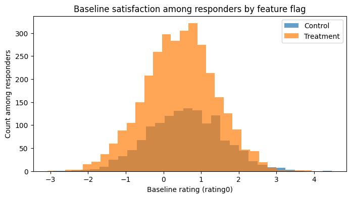
6.2 Baseline Satisfaction Among Responders
baseline_by_group = (responders
                      .groupby("feature_flag")["rating0"]
                      .mean())
baseline_by_group
feature_flag
0    0.5869
1    0.4404
Name: rating0, dtype: float64
If randomization still “held” inside the responder subset, baseline satisfaction (rating0)
would be similar between feature and control groups.
Instead, you will see that control responders typically have higher baseline satisfaction than treated responders.
That is selection bias created by conditioning on a collider (responded depends on both treatment and outcome).
6.3 Visualizing Baseline Rating Among Responders
plt.figure(figsize=(8,4))
plt.hist(responders.loc[responders.feature_flag == 0, "rating0"], bins=30, alpha=0.7, label="Control")
plt.hist(responders.loc[responders.feature_flag == 1, "rating0"], bins=30, alpha=0.7, label="Treatment")
plt.xlabel("Baseline rating (rating0)")
plt.ylabel("Count among responders")
plt.title("Baseline satisfaction among responders by feature flag")
plt.legend()
plt.show()
7. Summary
- We implemented a version-agnostic d-separation checker using only
networkx. - We used it to demonstrate:
- Chains, forks, colliders and how association flows.
- How backdoor paths create confounding and how to fix it with adjustment.
- How selection bias arises by conditioning on colliders (like survey responders), even in randomized experiments.