
Bayesian_campaign_decisioning_hillstrom_data
Applying Bayesian Models to Real Campaign Data
Uncertainty-aware personalization with practical decisioning
This notebook is written as a blog-style artifact for practitioners.
Its purpose is show how to:
- apply Bayesian ideas from Chapters 1–4 in practice
- validate the model instead of blindly trusting it
- interpret results correctly
- translate model output into decisioning
Business question
What is the effect of sending an email on conversion, and how should we target when some customer segments are sparse and noisy?
This notebook uses the public Hillstrom / MineThatData email campaign dataset.
#!pip install arviz
#!pip install pymc
#!pip install --upgrade arviz pymc pytensor
#!conda install -c conda-forge gxx
#!pip install pymc==5.10.0 arviz==0.16.1
#!conda activate base
#!conda install -c conda-forge m2w64-toolchain --solver=libmamba -v
import pytensor
print(pytensor.config.cxx)
"C:\Users\revan\minicondanew\Library\mingw-w64\bin\g++.EXE"
import warnings
warnings.filterwarnings("ignore")

import numpy as np
import pandas as pd
import matplotlib.pyplot as plt
import arviz as az
import pymc as pm

from sklearn.compose import ColumnTransformer
from sklearn.pipeline import Pipeline
from sklearn.preprocessing import OneHotEncoder, StandardScaler
from sklearn.impute import SimpleImputer
from sklearn.linear_model import LogisticRegression
from sklearn.metrics import roc_auc_score, log_loss

RANDOM_STATE = 42
np.random.seed(RANDOM_STATE)
1. Load the data
The notebook is written around the Hillstrom email campaign dataset.
If the public URL does not work in your environment, place the CSV next to the notebook as hillstrom.csv.
To keep the first blog focused, I collapse the two campaign variants into a single binary treatment:
treatment = 1if the customer received any emailtreatment = 0if the customer received no email
DATA_URL = "http://www.minethatdata.com/Kevin_Hillstrom_MineThatData_E-MailAnalytics_DataMiningChallenge_2008.03.20.csv"
LOCAL_PATH = "hillstrom.csv"

try:
    df = pd.read_csv(DATA_URL)
    print("Loaded from URL.")
except Exception as e:
    print("URL load failed:", e)
    df = pd.read_csv(LOCAL_PATH)
    print("Loaded from local file.")

df.columns = [c.strip().lower() for c in df.columns]
print(df.shape)
df.head()
Loaded from URL.
(64000, 12)
| recency | history_segment | history | mens | womens | zip_code | newbie | channel | segment | visit | conversion | spend | |
|---|---|---|---|---|---|---|---|---|---|---|---|---|
| 0 | 10 | 2) $100 - $200 | 142.44 | 1 | 0 | Surburban | 0 | Phone | Womens E-Mail | 0 | 0 | 0.0 |
| 1 | 6 | 3) $200 - $350 | 329.08 | 1 | 1 | Rural | 1 | Web | No E-Mail | 0 | 0 | 0.0 |
| 2 | 7 | 2) $100 - $200 | 180.65 | 0 | 1 | Surburban | 1 | Web | Womens E-Mail | 0 | 0 | 0.0 |
| 3 | 9 | 5) $500 - $750 | 675.83 | 1 | 0 | Rural | 1 | Web | Mens E-Mail | 0 | 0 | 0.0 |
| 4 | 2 | 1) $0 - $100 | 45.34 | 1 | 0 | Urban | 0 | Web | Womens E-Mail | 0 | 0 | 0.0 |
2. Define treatment, outcome, and pre-treatment features
I use conversion as the main outcome because:
- Bayesian logistic regression is easy to explain
- posterior probabilities are intuitive
- decision thresholds are easier to justify
I restrict predictors to pre-treatment variables only. That is basic causal discipline and keeps the model interpretable.
work = df.copy()

work["treatment"] = (work["segment"] != "No E-Mail").astype(int)
work["y"] = work["conversion"].astype(int)

work["history_segment"] = work["history_segment"].astype(str).str.strip()
work["zip_code"] = work["zip_code"].astype(str).str.strip()
work["channel"] = work["channel"].astype(str).str.strip()

feature_cols = [
    "recency", "history", "mens", "womens", "newbie",
    "zip_code", "channel", "history_segment"
]

work = work[feature_cols + ["treatment", "y"]].copy()
work.head()
| recency | history | mens | womens | newbie | zip_code | channel | history_segment | treatment | y | |
|---|---|---|---|---|---|---|---|---|---|---|
| 0 | 10 | 142.44 | 1 | 0 | 0 | Surburban | Phone | 2) $100 - $200 | 1 | 0 |
| 1 | 6 | 329.08 | 1 | 1 | 1 | Rural | Web | 3) $200 - $350 | 0 | 0 |
| 2 | 7 | 180.65 | 0 | 1 | 1 | Surburban | Web | 2) $100 - $200 | 1 | 0 |
| 3 | 9 | 675.83 | 1 | 0 | 1 | Rural | Web | 5) $500 - $750 | 1 | 0 |
| 4 | 2 | 45.34 | 1 | 0 | 0 | Urban | Web | 1) $0 - $100 | 1 | 0 |
3. Quick descriptive readout
This is not the final causal answer. It is just a reality check before modeling.
raw_summary = work.groupby("treatment")["y"].agg(["mean", "sum", "count"])
raw_summary["conversion_rate_pct"] = 100 * raw_summary["mean"]
raw_summary
| mean | sum | count | conversion_rate_pct | |
|---|---|---|---|---|
| treatment | ||||
| 0 | 0.005726 | 122 | 21306 | 0.572609 |
| 1 | 0.010681 | 456 | 42694 | 1.068066 |
Interpretation
This tells me whether treated and untreated groups move in the direction I would expect.
But raw rates are not enough for a serious decision system:
- they do not make uncertainty explicit
- they do not stabilize small segments
- they are weak support for action when slices are noisy
4. Classical baseline
I include a standard logistic model as a benchmark.
The point is not to say classical models are bad. The point is to show what Bayesian modeling adds.
numeric_cols = ["recency", "history", "mens", "womens", "newbie", "treatment"]
categorical_cols = ["zip_code", "channel", "history_segment"]

X = work[numeric_cols + categorical_cols]
y = work["y"]

preprocess = ColumnTransformer(
    transformers=[
        ("num", Pipeline([
            ("imputer", SimpleImputer(strategy="median")),
            ("scaler", StandardScaler()),
        ]), numeric_cols),
        ("cat", Pipeline([
            ("imputer", SimpleImputer(strategy="most_frequent")),
            ("ohe", OneHotEncoder(drop="first", handle_unknown="ignore")),
        ]), categorical_cols),
    ]
)

baseline = Pipeline([
    ("prep", preprocess),
    ("model", LogisticRegression(max_iter=2000, random_state=RANDOM_STATE)),
])

baseline.fit(X, y)
baseline_proba = baseline.predict_proba(X)[:, 1]

print("Baseline log loss:", round(log_loss(y, baseline_proba), 5))
print("Baseline AUC:", round(roc_auc_score(y, baseline_proba), 5))
Baseline log loss: 0.05027
Baseline AUC: 0.64399
Interpretation
The baseline is useful, but it still leaves open the business questions I care about:
- How uncertain is the campaign effect?
- Which segments are promising but too noisy to trust?
- What targeting rule would I actually deploy?
That is the gap Bayesian modeling helps fill.
5. Build a compact Bayesian modeling table
For the blog, I use a compact but realistic specification. The idea is to keep the notebook:
- practical
- interpretable
- fast enough to run without turning the blog into an engineering exercise
bayes_df = work[["recency", "history", "mens", "womens", "newbie", "history_segment", "treatment", "y"]].copy()

bayes_df["group"] = bayes_df["history_segment"].astype("category")
bayes_df["group_idx"] = bayes_df["group"].cat.codes
group_names = bayes_df["group"].cat.categories.tolist()

for col in ["recency", "history"]:
    bayes_df[f"{col}_z"] = (bayes_df[col] - bayes_df[col].mean()) / bayes_df[col].std()

MAX_N = 15000
if len(bayes_df) > MAX_N:
    bayes_df = bayes_df.sample(MAX_N, random_state=RANDOM_STATE).reset_index(drop=True)

print(bayes_df.shape)
bayes_df.head()
(15000, 12)
| recency | history | mens | womens | newbie | history_segment | treatment | y | group | group_idx | recency_z | history_z | |
|---|---|---|---|---|---|---|---|---|---|---|---|---|
| 0 | 9 | 64.85 | 1 | 0 | 1 | 1) $0 - $100 | 1 | 0 | 1) $0 - $100 | 0 | 0.922646 | -0.691898 |
| 1 | 1 | 144.12 | 0 | 1 | 0 | 2) $100 - $200 | 1 | 0 | 2) $100 - $200 | 1 | -1.358121 | -0.382441 |
| 2 | 1 | 734.25 | 0 | 1 | 1 | 5) $500 - $750 | 1 | 0 | 5) $500 - $750 | 4 | -1.358121 | 1.921327 |
| 3 | 4 | 1321.26 | 1 | 0 | 1 | 7) $1,000 + | 1 | 0 | 7) $1,000 + | 6 | -0.502833 | 4.212915 |
| 4 | 2 | 261.23 | 1 | 1 | 1 | 3) $200 - $350 | 1 | 0 | 3) $200 - $350 | 2 | -1.073025 | 0.074736 |
6. Prior predictive thinking
Before fitting the model, I ask:
If my priors were true, what sort of conversion rates would they imply?
This is practical Bayesian modeling. Priors are assumptions, so they should generate plausible business outcomes.
with pm.Model() as prior_model:
    alpha = pm.Normal("alpha", mu=-3.0, sigma=1.0)
    beta_t = pm.Normal("beta_t", mu=0.0, sigma=0.5)
    beta_recency = pm.Normal("beta_recency", mu=0.0, sigma=0.5)
    beta_history = pm.Normal("beta_history", mu=0.0, sigma=0.5)
    beta_mens = pm.Normal("beta_mens", mu=0.0, sigma=0.5)
    beta_womens = pm.Normal("beta_womens", mu=0.0, sigma=0.5)
    beta_newbie = pm.Normal("beta_newbie", mu=0.0, sigma=0.5)

    logit_p = (
        alpha
        + beta_t * bayes_df["treatment"].values
        + beta_recency * bayes_df["recency_z"].values
        + beta_history * bayes_df["history_z"].values
        + beta_mens * bayes_df["mens"].values
        + beta_womens * bayes_df["womens"].values
        + beta_newbie * bayes_df["newbie"].values
    )

    p = pm.Deterministic("p", pm.math.sigmoid(logit_p))
    prior_pred = pm.sample_prior_predictive(samples=500, random_seed=RANDOM_STATE)

prior_p = prior_pred.prior["p"].values.reshape(-1)

plt.figure(figsize=(8, 4))
plt.hist(prior_p, bins=50)
plt.title("Prior predictive implied conversion probabilities")
plt.xlabel("Implied probability")
plt.ylabel("Count")
plt.show()
Sampling: [alpha, beta_history, beta_mens, beta_newbie, beta_recency, beta_t, beta_womens]
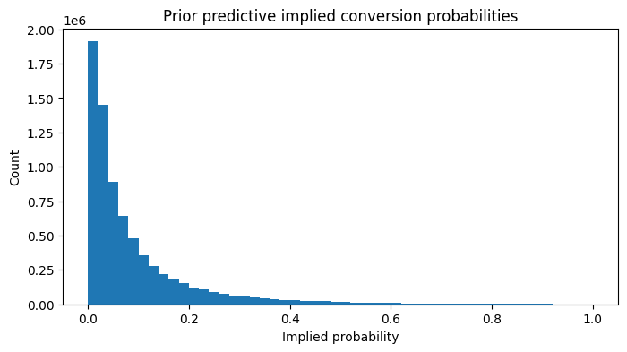
Interpretation
What I want from this check:
- mostly low conversion probabilities
- enough flexibility for treatment and features to matter
- no prior-driven nonsense like huge probabilities for routine customers
This is one of the easiest ways to check if the prior-related assumptions are acceptable.
7. Bayesian logistic regression: overall campaign effect
Now I fit a pooled Bayesian logistic model.
This gives me:
- a posterior distribution over the treatment effect
- a natural way to ask probability-style questions
- a cleaner bridge from model output to action
coords = {"obs_id": np.arange(len(bayes_df))}

with pm.Model(coords=coords) as pooled_model:
    treatment = pm.Data("treatment", bayes_df["treatment"].values, dims="obs_id")
    recency_z = pm.Data("recency_z", bayes_df["recency_z"].values, dims="obs_id")
    history_z = pm.Data("history_z", bayes_df["history_z"].values, dims="obs_id")
    mens = pm.Data("mens", bayes_df["mens"].values, dims="obs_id")
    womens = pm.Data("womens", bayes_df["womens"].values, dims="obs_id")
    newbie = pm.Data("newbie", bayes_df["newbie"].values, dims="obs_id")
    y_obs = pm.Data("y_obs", bayes_df["y"].values, dims="obs_id")

    alpha = pm.Normal("alpha", mu=-3.0, sigma=1.0)
    beta_t = pm.Normal("beta_t", mu=0.0, sigma=0.5)
    beta_recency = pm.Normal("beta_recency", mu=0.0, sigma=0.5)
    beta_history = pm.Normal("beta_history", mu=0.0, sigma=0.5)
    beta_mens = pm.Normal("beta_mens", mu=0.0, sigma=0.5)
    beta_womens = pm.Normal("beta_womens", mu=0.0, sigma=0.5)
    beta_newbie = pm.Normal("beta_newbie", mu=0.0, sigma=0.5)

    logit_p = (
        alpha
        + beta_t * treatment
        + beta_recency * recency_z
        + beta_history * history_z
        + beta_mens * mens
        + beta_womens * womens
        + beta_newbie * newbie
    )

    p = pm.Deterministic("p", pm.math.sigmoid(logit_p), dims="obs_id")
    outcome = pm.Bernoulli("outcome", p=p, observed=y_obs, dims="obs_id")

    idata_pooled = pm.sample(
        draws=1000,
        tune=1500, #1000
        chains=4,
        target_accept=0.95, #0.90
        max_treedepth=12, #None
        random_seed=RANDOM_STATE,
        return_inferencedata=True,
    )
Initializing NUTS using jitter+adapt_diag...
Multiprocess sampling (4 chains in 4 jobs)
NUTS: [alpha, beta_t, beta_recency, beta_history, beta_mens, beta_womens, beta_newbie]


Output()
Sampling 4 chains for 1_500 tune and 1_000 draw iterations (6_000 + 4_000 draws total) took 284 seconds.
az.summary(
    idata_pooled,
    var_names=["alpha", "beta_t", "beta_recency", "beta_history", "beta_mens", "beta_womens", "beta_newbie"],
    round_to=3,
)
| mean | sd | hdi_3% | hdi_97% | mcse_mean | mcse_sd | ess_bulk | ess_tail | r_hat | |
|---|---|---|---|---|---|---|---|---|---|
| alpha | -5.264 | 0.276 | -5.796 | -4.766 | 0.007 | 0.004 | 1459.918 | 2271.160 | 1.004 |
| beta_t | 0.444 | 0.177 | 0.111 | 0.765 | 0.003 | 0.003 | 3096.992 | 2597.386 | 1.002 |
| beta_recency | -0.162 | 0.086 | -0.337 | -0.006 | 0.001 | 0.001 | 3491.311 | 2748.742 | 1.001 |
| beta_history | 0.177 | 0.074 | 0.041 | 0.318 | 0.001 | 0.001 | 2695.236 | 2395.130 | 1.001 |
| beta_mens | 0.476 | 0.210 | 0.093 | 0.876 | 0.005 | 0.003 | 1799.914 | 2728.155 | 1.002 |
| beta_womens | 0.396 | 0.213 | 0.008 | 0.811 | 0.005 | 0.003 | 1970.892 | 2451.781 | 1.003 |
| beta_newbie | -0.424 | 0.163 | -0.763 | -0.136 | 0.003 | 0.003 | 3121.234 | 2414.047 | 1.001 |
beta_t_samples = idata_pooled.posterior["beta_t"].values.reshape(-1)
prob_positive = (beta_t_samples > 0).mean()
print(f"Posterior P(email effect > 0 on log-odds scale): {prob_positive:.3f}")
Posterior P(email effect > 0 on log-odds scale): 0.996
Interpretation
This is where the Bayesian model becomes genuinely useful for campaign decisioning.
A classical workflow might stop at a coefficient and maybe an interval.
Here I can ask:
What is the probability that the campaign effect is actually positive?
That is much closer to how targeting decisions are made in practice.
8. Posterior versus posterior predictive
This distinction matters.
- Posterior = uncertainty about parameters
- Posterior predictive = uncertainty about future outcomes
In practice, the second object is what feeds prediction and action.
with pooled_model:
    post_pred_pooled = pm.sample_posterior_predictive(
        idata_pooled,
        var_names=["outcome", "p"],
        random_seed=RANDOM_STATE,
    )

idata_pooled.extend(post_pred_pooled)
Sampling: [outcome]


Output()
pp_y = idata_pooled.posterior_predictive["outcome"].values
pp_rate = pp_y.mean(axis=(0, 2))
observed_rate = bayes_df["y"].mean()

plt.figure(figsize=(8, 4))
plt.hist(pp_rate, bins=40)
plt.axvline(observed_rate, linestyle="--")
plt.title("Posterior predictive check: overall conversion rate")
plt.xlabel("Predicted conversion rate from posterior predictive draws")
plt.ylabel("Count")
plt.show()

print("Observed conversion rate:", round(observed_rate, 5))
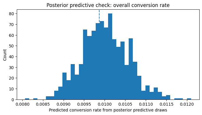
Observed conversion rate: 0.00987
Interpretation
This is one of the most practical validation checks in the notebook.
I am asking:
Can the fitted model regenerate data with broad characteristics similar to what I actually observed?
If not, I should not trust its decision recommendations. Since observed coversion rate lies comfortably in the range shown in the histogram, this result passes the check.
9. Hierarchical modeling for personalization
A single global treatment effect is useful, but personalization systems usually need more.
They ask:
- which groups respond more?
- which groups are too noisy to trust?
- where should we target more aggressively?
A naive slice-by-slice estimate can be unstable. A hierarchical model improves this through partial pooling and shrinkage.
For interpretability, I model treatment-effect heterogeneity only across history (prior-spend) segments while controlling for other customer attributes through shared fixed effects. This allows the Bayesian hierarchy to capture meaningful business segmentation without exploding the number of sparse subgroup combinations.
naive_seg = (
    bayes_df.groupby(["group", "treatment"])["y"]
    .agg(["mean", "count", "sum"])
    .reset_index()
)
#raw lift is the difference in mean conversion rates of treatment/control customers  within each segment
pivot_rate = naive_seg.pivot(index="group", columns="treatment", values="mean")
pivot_n = naive_seg.pivot(index="group", columns="treatment", values="count")
naive_lift = (pivot_rate[1] - pivot_rate[0]).rename("raw_lift")
naive_lift = pd.concat([naive_lift, pivot_n.add_prefix("n_treat_")], axis=1)
naive_lift.sort_values("raw_lift", ascending=False)
| raw_lift | n_treat_0 | n_treat_1 | |
|---|---|---|---|
| group | |||
| 4) $350 - $500 | 0.011695 | 523 | 988 |
| 5) $500 - $750 | 0.009376 | 395 | 766 |
| 3) $200 - $350 | 0.007777 | 942 | 1913 |
| 6) $750 - $1,000 | 0.007264 | 160 | 296 |
| 1) $0 - $100 | 0.002492 | 1824 | 3638 |
| 2) $100 - $200 | 0.002194 | 1074 | 2185 |
| 7) $1,000 + | -0.003850 | 87 | 209 |
coords_h = {
    "obs_id": np.arange(len(bayes_df)),
    "group": group_names,
}

with pm.Model(coords=coords_h) as hierarchical_model:
    treatment = pm.Data("treatment", bayes_df["treatment"].values, dims="obs_id")
    recency_z = pm.Data("recency_z", bayes_df["recency_z"].values, dims="obs_id")
    history_z = pm.Data("history_z", bayes_df["history_z"].values, dims="obs_id")
    mens = pm.Data("mens", bayes_df["mens"].values, dims="obs_id")
    womens = pm.Data("womens", bayes_df["womens"].values, dims="obs_id")
    newbie = pm.Data("newbie", bayes_df["newbie"].values, dims="obs_id")
    group_idx = pm.Data("group_idx", bayes_df["group_idx"].values, dims="obs_id")
    y_obs = pm.Data("y_obs", bayes_df["y"].values, dims="obs_id")

    alpha = pm.Normal("alpha", mu=-3.0, sigma=1.0) #+> baseline probability is low, roughly in single digit % sigma(-3)~0.047
    beta_recency = pm.Normal("beta_recency", mu=0.0, sigma=0.5)
    beta_history = pm.Normal("beta_history", mu=0.0, sigma=0.5)
    beta_mens = pm.Normal("beta_mens", mu=0.0, sigma=0.5)
    beta_womens = pm.Normal("beta_womens", mu=0.0, sigma=0.5)
    beta_newbie = pm.Normal("beta_newbie", mu=0.0, sigma=0.5)

   # mu_t = pm.Normal("mu_t", mu=0.0, sigma=0.5)
   # sigma_t = pm.HalfNormal("sigma_t", sigma=0.5)
   # beta_t_group = pm.Normal("beta_t_group", mu=mu_t, sigma=sigma_t, dims="group")
   #I use a non-centered hierarchical parameterization to improve Bayesian sampler stability.
    #This reformulation preserves the same statistical model while reducing divergences and improving convergence in sparse-segment settings.

    mu_t = pm.Normal("mu_t", mu=0.0, sigma=0.5)
    sigma_t = pm.HalfNormal("sigma_t", sigma=0.5)
    z_t = pm.Normal("z_t", mu=0.0, sigma=1.0, dims="group")
    beta_t_group = pm.Deterministic("beta_t_group", mu_t + z_t * sigma_t, dims="group")

    logit_p = (
        alpha
        + beta_t_group[group_idx] * treatment
        + beta_recency * recency_z
        + beta_history * history_z
        + beta_mens * mens
        + beta_womens * womens
        + beta_newbie * newbie
    )

    p = pm.Deterministic("p", pm.math.sigmoid(logit_p), dims="obs_id")
    outcome = pm.Bernoulli("outcome", p=p, observed=y_obs, dims="obs_id")

    idata_h = pm.sample(
        draws=1000,
        tune=1000,
        chains=4,
        target_accept=0.92,
        random_seed=RANDOM_STATE,
        return_inferencedata=True,
    )
Initializing NUTS using jitter+adapt_diag...
Multiprocess sampling (4 chains in 4 jobs)
NUTS: [alpha, beta_recency, beta_history, beta_mens, beta_womens, beta_newbie, mu_t, sigma_t, z_t]


Output()
Sampling 4 chains for 1_000 tune and 1_000 draw iterations (4_000 + 4_000 draws total) took 299 seconds.
To stabilize sampling in the hierarchical treatment-effect model, I use a non-centered parameterization for segment-level treatment effects.
Instead of sampling each segment treatment effect directly from:
β_t_group ~ Normal(μ_t, σ_t)
I reparameterize as:
z_t ~ Normal(0, 1)
β_t_group = μ_t + z_t × σ_t
This mathematically represents the same hierarchical model, but often samples much more efficiently in Bayesian hierarchical settings.
Why this matters:
- Direct centered parameterization can create strong posterior correlations between group effects and hierarchy parameters.
- That often leads to divergences, poor effective sample size, and slow NUTS convergence.
- Non-centered parameterization reduces this geometry problem and improves sampler stability.
This is especially useful when:
- Some groups are sparse
- Hierarchical variance is small
- Partial pooling is strong
az.summary(idata_h, var_names=["mu_t", "sigma_t", "beta_t_group"], round_to=3)
| mean | sd | hdi_3% | hdi_97% | mcse_mean | mcse_sd | ess_bulk | ess_tail | r_hat | |
|---|---|---|---|---|---|---|---|---|---|
| mu_t | 0.427 | 0.194 | 0.084 | 0.812 | 0.003 | 0.003 | 3285.879 | 2711.547 | 1.003 |
| sigma_t | 0.182 | 0.142 | 0.000 | 0.437 | 0.003 | 0.002 | 1682.274 | 1786.548 | 1.000 |
| beta_t_group[1) $0 - $100] | 0.439 | 0.203 | 0.057 | 0.825 | 0.003 | 0.003 | 4646.861 | 3169.858 | 1.001 |
| beta_t_group[2) $100 - $200] | 0.353 | 0.227 | -0.112 | 0.745 | 0.004 | 0.003 | 3561.391 | 2925.678 | 1.002 |
| beta_t_group[3) $200 - $350] | 0.419 | 0.212 | 0.002 | 0.802 | 0.003 | 0.003 | 4833.690 | 3483.099 | 1.000 |
| beta_t_group[4) $350 - $500] | 0.560 | 0.238 | 0.123 | 1.003 | 0.004 | 0.003 | 3055.097 | 3139.759 | 1.001 |
| beta_t_group[5) $500 - $750] | 0.500 | 0.240 | 0.052 | 0.953 | 0.004 | 0.003 | 3675.060 | 3178.447 | 1.001 |
| beta_t_group[6) $750 - $1,000] | 0.400 | 0.266 | -0.107 | 0.895 | 0.004 | 0.004 | 3962.511 | 3423.523 | 1.002 |
| beta_t_group[7) $1,000 +] | 0.397 | 0.277 | -0.148 | 0.902 | 0.004 | 0.005 | 3771.996 | 3328.389 | 1.001 |
R-hat ≈ 1.000–1.003 Excellent Effective Sample Size ESS mostly 3000–4800
posterior samples are now reliable enough to interpret as
R-hat < 1.01 ESS > 400 (100 × number_of_chains) Divergences = 0
beta_group = idata_h.posterior["beta_t_group"].stack(sample=("chain", "draw")).values

hier = pd.DataFrame({
    "group": group_names,
    "post_mean_logodds_effect": beta_group.mean(axis=1),
    "post_prob_positive": (beta_group > 0).mean(axis=1),
    "post_p10": np.quantile(beta_group, 0.10, axis=1),
    "post_p90": np.quantile(beta_group, 0.90, axis=1),
})

comparison = naive_lift.reset_index().merge(hier, on="group", how="left")
comparison.sort_values("post_prob_positive", ascending=False)
| group | raw_lift | n_treat_0 | n_treat_1 | post_mean_logodds_effect | post_prob_positive | post_p10 | post_p90 | |
|---|---|---|---|---|---|---|---|---|
| 3 | 4) $350 - $500 | 0.011695 | 523 | 988 | 0.560170 | 0.99675 | 0.265967 | 0.884051 |
| 4 | 5) $500 - $750 | 0.009376 | 395 | 766 | 0.500078 | 0.98700 | 0.204615 | 0.808252 |
| 0 | 1) $0 - $100 | 0.002492 | 1824 | 3638 | 0.439379 | 0.98375 | 0.184999 | 0.697553 |
| 2 | 3) $200 - $350 | 0.007777 | 942 | 1913 | 0.418892 | 0.97775 | 0.149250 | 0.681799 |
| 5 | 6) $750 - $1,000 | 0.007264 | 160 | 296 | 0.399655 | 0.93500 | 0.070966 | 0.726050 |
| 6 | 7) $1,000 + | -0.003850 | 87 | 209 | 0.397161 | 0.92925 | 0.059925 | 0.724186 |
| 1 | 2) $100 - $200 | 0.002194 | 1074 | 2185 | 0.353053 | 0.92825 | 0.053629 | 0.628934 |
- The hierarchical Bayesian model identified statistically credible heterogeneity in treatment response across customer value segments. Segment-level treatment effects were partially pooled toward the population mean, reducing noise relative to naïve segment estimates while preserving meaningful differences where supported by data.
Interpretation
This is where the approach becomes especially useful for personalization.
The raw segment effects are easy to compute but often too noisy to trust. The hierarchical model provides:
- stable segment-level estimates
- a direct probability that each segment benefits
- much less temptation to chase random extremes from thin data
The posterior probability of positive treatment effect exceeds 92% across all customer history segments, indicating broad evidence that email campaigns improve conversion. However, the magnitude of expected benefit varies by segment, suggesting that while blanket suppression is not warranted, prioritization by expected incremental value remains appropriate.
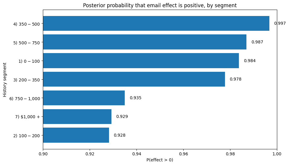
10. Turning model output into decisions
A model is only useful if it can support action.
Below is a simple policy-style interpretation:
- high posterior probability of benefit -> target confidently
- moderate posterior probability -> promising, but monitor or test more
- weak posterior probability -> de-prioritize for now
plot_df = comparison.sort_values("post_prob_positive", ascending=True)

plt.figure(figsize=(10, 6))
plt.barh(plot_df["group"].astype(str), plot_df["post_prob_positive"])
plt.axvline(0.8, linestyle="--")
plt.title("Posterior probability that email effect is positive, by segment")
plt.xlim(0.90, 1.0)
plt.xlabel("P(effect > 0)")
plt.ylabel("History segment")
for i, v in enumerate(plot_df["post_prob_positive"]):
    plt.text(v + 0.002, i, f"{v:.3f}", va="center")
plt.show()
decision_df = comparison[["group", "post_prob_positive", "post_mean_logodds_effect", "post_p10", "post_p90"]].copy()

decision_df["recommended_action"] = np.select(
    [
        decision_df["post_prob_positive"] >= 0.90,
        decision_df["post_prob_positive"].between(0.70, 0.90, inclusive="left"),
    ],
    [
        "Target confidently",
        "Promising but monitor / test more",
    ],
    default="Weak evidence: deprioritize for now",
)

decision_df.sort_values("post_prob_positive", ascending=False)
| group | post_prob_positive | post_mean_logodds_effect | post_p10 | post_p90 | recommended_action | |
|---|---|---|---|---|---|---|
| 3 | 4) $350 - $500 | 0.99675 | 0.560170 | 0.265967 | 0.884051 | Target confidently |
| 4 | 5) $500 - $750 | 0.98700 | 0.500078 | 0.204615 | 0.808252 | Target confidently |
| 0 | 1) $0 - $100 | 0.98375 | 0.439379 | 0.184999 | 0.697553 | Target confidently |
| 2 | 3) $200 - $350 | 0.97775 | 0.418892 | 0.149250 | 0.681799 | Target confidently |
| 5 | 6) $750 - $1,000 | 0.93500 | 0.399655 | 0.070966 | 0.726050 | Target confidently |
| 6 | 7) $1,000 + | 0.92925 | 0.397161 | 0.059925 | 0.724186 | Target confidently |
| 1 | 2) $100 - $200 | 0.92825 | 0.353053 | 0.053629 | 0.628934 | Target confidently |
Interpretation A naïve segment-level uplift table would have suggested suppressing email to the highest-value customers (1000$+ group) because observed raw lift was negative in that sparse segment as shown in a previous table. However, the hierarchical Bayesian model identified that the apparent negative lift was likely noise caused by limited sample size. After partial pooling, posterior probability of positive treatment effect for that segment remained above 92%. This demonstrates how Bayesian hierarchical models prevent overreaction to noisy segment-level estimates in personalization systems. This is the practical payoff.
The model is not just producing parameters. It is supporting a targeting rule that explicitly accounts for uncertainty.
That is one of the biggest reasons Bayesian models are attractive in campaign analytics and personalization systems.
effect_df = comparison.sort_values("post_mean_logodds_effect", ascending=True).copy()

plt.figure(figsize=(10, 6))
plt.errorbar(
    x=effect_df["post_mean_logodds_effect"],
    y=effect_df["group"].astype(str),
    xerr=[
        effect_df["post_mean_logodds_effect"] - effect_df["post_p10"],
        effect_df["post_p90"] - effect_df["post_mean_logodds_effect"]
    ],
    fmt="o"
)

plt.axvline(0, linestyle="--")
plt.title("Posterior treatment effect by segment on log-odds scale")
plt.xlabel("Posterior treatment effect (log-odds scale)")
plt.ylabel("History segment")
plt.show()
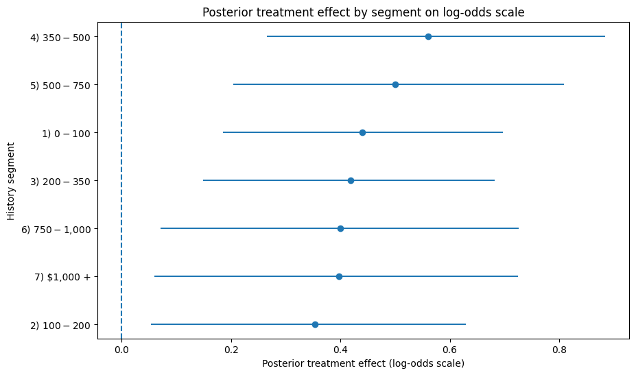
These effects are shown on the log-odds scale from the Bayesian logistic model, so they are useful for relative segment ranking but not yet a direct measure of business lift. I use two complementary views of segment-level treatment effects. The first plot shows the posterior probability that email has a positive effect for each segment, which is useful for suppression or go/no-go decisions. The second plot shows posterior mean treatment effect with uncertainty intervals, which is more useful for prioritizing segments by expected incremental impact.
import numpy as np
import pandas as pd

# Pull posterior draws
posterior = idata_h.posterior

alpha_s = posterior["alpha"].values.reshape(-1)
beta_recency_s = posterior["beta_recency"].values.reshape(-1)
beta_history_s = posterior["beta_history"].values.reshape(-1)
beta_mens_s = posterior["beta_mens"].values.reshape(-1)
beta_womens_s = posterior["beta_womens"].values.reshape(-1)
beta_newbie_s = posterior["beta_newbie"].values.reshape(-1)

# shape: (n_groups, n_samples)
beta_t_group_s = posterior["beta_t_group"].stack(sample=("chain", "draw")).values

# Build one row per segment using average feature values inside that segment.
segment_profiles = (
    bayes_df.groupby("group")
    .agg(
        recency_z=("recency_z", "mean"),
        history_z=("history_z", "mean"),
        mens=("mens", "mean"),
        womens=("womens", "mean"),
        newbie=("newbie", "mean"),
        n=("y", "size"),
        observed_conversion=("y", "mean"),
    )
    .reset_index()
)

rows = []

for g_idx, row in segment_profiles.iterrows():
    # Linear predictor under control
    eta_control = (
        alpha_s
        + beta_recency_s * row["recency_z"]
        + beta_history_s * row["history_z"]
        + beta_mens_s * row["mens"]
        + beta_womens_s * row["womens"]
        + beta_newbie_s * row["newbie"]
    )

    # Add treatment effect for treated scenario
    eta_treat = eta_control + beta_t_group_s[g_idx, :]

    # Convert log-odds to probabilities
    p_control = 1 / (1 + np.exp(-eta_control))
    p_treat = 1 / (1 + np.exp(-eta_treat))
    uplift = p_treat - p_control

    rows.append({
        "group": row["group"],
        "n": row["n"],
        "observed_conversion": row["observed_conversion"],
        "post_control_mean": p_control.mean(),
        "post_treat_mean": p_treat.mean(),
        "post_uplift_mean": uplift.mean(),
        "post_uplift_p10": np.quantile(uplift, 0.10),
        "post_uplift_p90": np.quantile(uplift, 0.90),
        "prob_uplift_positive": (uplift > 0).mean(),
    })

uplift_df = pd.DataFrame(rows).sort_values("post_uplift_mean", ascending=False)
uplift_df
| group | n | observed_conversion | post_control_mean | post_treat_mean | post_uplift_mean | post_uplift_p10 | post_uplift_p90 | prob_uplift_positive | |
|---|---|---|---|---|---|---|---|---|---|
| 6 | 7) $1,000 + | 296 | 0.020270 | 0.015221 | 0.022415 | 0.007193 | 0.000990 | 0.013722 | 0.92925 |
| 3 | 4) $350 - $500 | 1511 | 0.017207 | 0.009198 | 0.016049 | 0.006850 | 0.003115 | 0.011291 | 0.99675 |
| 4 | 5) $500 - $750 | 1161 | 0.013781 | 0.008203 | 0.013473 | 0.005271 | 0.002057 | 0.008803 | 0.98700 |
| 5 | 6) $750 - $1,000 | 456 | 0.010965 | 0.010519 | 0.015694 | 0.005176 | 0.000820 | 0.009574 | 0.93500 |
| 2 | 3) $200 - $350 | 2855 | 0.009457 | 0.007654 | 0.011575 | 0.003922 | 0.001338 | 0.006472 | 0.97775 |
| 0 | 1) $0 - $100 | 5462 | 0.008239 | 0.005577 | 0.008583 | 0.003006 | 0.001281 | 0.004754 | 0.98375 |
| 1 | 2) $100 - $200 | 3259 | 0.007057 | 0.006177 | 0.008776 | 0.002600 | 0.000363 | 0.004645 | 0.92825 |
plot_df = uplift_df.sort_values("post_treat_mean", ascending=True)

y_pos = np.arange(len(plot_df))

plt.figure(figsize=(10, 6))
plt.barh(y_pos - 0.2, plot_df["post_control_mean"], height=0.4, label="Control")
plt.barh(y_pos + 0.2, plot_df["post_treat_mean"], height=0.4, label="Treatment")

plt.yticks(y_pos, plot_df["group"].astype(str))
plt.xlabel("Posterior mean conversion probability")
plt.ylabel("History segment")
plt.title("Posterior predicted conversion by segment")
plt.legend()
plt.show()
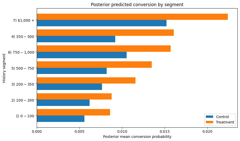
Rather than ranking segments purely on treatment effect coefficient size or raw observed lift, I convert posterior segment effects into expected conversion under treatment and control. This makes the output directly useful for decisioning: it tells me not only whether a segment is likely to benefit, but also how much incremental conversion I should expect if I target it.
While all segments show positive expected uplift, the model suggests prioritizing the highest-history and mid-high-history customers first, with the $1,000+ segment exhibiting the largest expected incremental conversion despite relatively sparse data. This ranking differs materially from naïve raw-lift and coefficient-based ranking, highlighting the importance of converting posterior treatment effects into expected business uplift before decisioning.
plot_df = uplift_df.sort_values("post_uplift_mean", ascending=True).copy()

plt.figure(figsize=(10, 6))
plt.errorbar(
x=plot_df["post_uplift_mean"],
y=plot_df["group"].astype(str),
xerr=[
plot_df["post_uplift_mean"] - plot_df["post_uplift_p10"],
plot_df["post_uplift_p90"] - plot_df["post_uplift_mean"]
],
fmt="o"
)

for i, row in plot_df.reset_index(drop=True).iterrows():
    plt.text(
    row["post_uplift_mean"] + 0.0001,
    i,
    f"{row['post_uplift_mean']:.4f}",
    va="center"
    )

plt.axvline(0, linestyle="--")
plt.title("Posterior expected uplift by segment")
plt.xlabel("Expected uplift in conversion probability")
plt.ylabel("History segment")
plt.show()
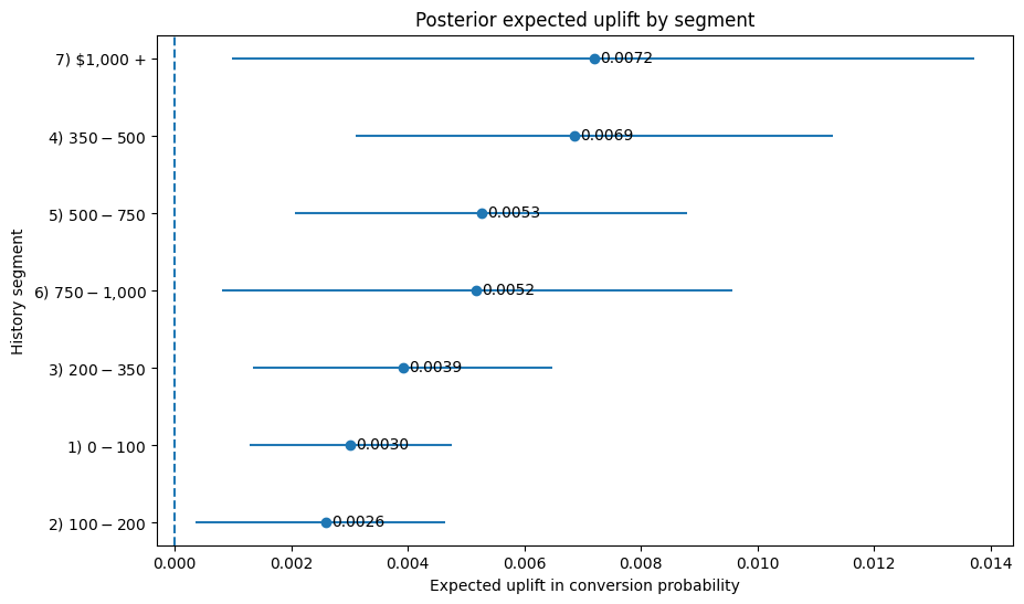
While all segments show positive expected uplift, the model suggests prioritizing the highest-history and mid-high-history customers first, with the $1,000+ segment exhibiting the largest expected incremental conversion despite relatively sparse data. This ranking differs materially from naïve raw-lift and coefficient-based ranking, highlighting the importance of converting posterior treatment effects into expected business uplift before decisioning.
This plot translates posterior treatment effects into expected incremental conversion by segment, which is more directly useful for campaign prioritization than coefficient estimates on the log-odds scale. The point estimate shows expected uplift, while the interval reflects posterior uncertainty.
11. Final takeaways
This post shows how Bayesian Causal modeling can be applied in a real campaign decisioning setting-not just to estimate treatment effects, but to make better targeting decisions under uncertainty. Specifically, I:
- estimated heterogeneous email treatment effects across customer spend segments
- used hierarchical partial pooling to stabilize sparse segment estimates
- validated convergence and sampling diagnostics before trusting the posterior
- translated posterior treatment effects from log-odds into expected conversion uplift
- ranked segments using expected incremental conversion rather than naïve observed lift
- quantified uncertainty using posterior uplift intervals and probability uplift is positive
Practical Lesson:
Bayesian uplift models are most valuable when segment-level treatment effects are noisy, sparse, or high stakes enough that uncertainty should influence targeting decisions—not just point estimates